The Connection Between Physical Diffusion and AI Diffusion Models

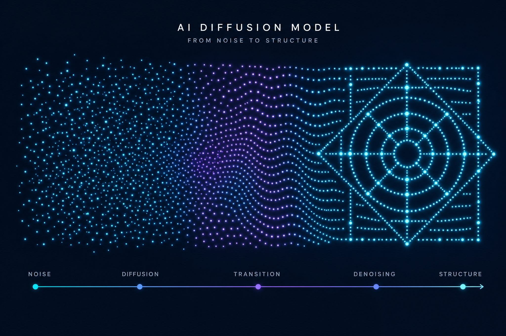
In 1855, Adolf Fick wrote down two equations describing how ink spreads through water. In 2015, exactly 160 years later, a Stanford PhD student named Jascha Sohl-Dickstein published a paper using those same equations to generate images from noise. The lineage is not metaphorical. The mathematical machinery of AI diffusion models — the score functions, the Langevin dynamics, the Fokker-Planck equation — was lifted directly from statistical physics. The most powerful image generation technology in the world is, at its mathematical core, a 19th-century theory of how particles spread.

This article traces that connection in full. It is the capstone of our series on diffusion, and it draws on every concept we've covered: Fick's laws, Brownian motion, the Fokker-Planck equation, and the denoising process that powers modern AI. If you've read those articles, you have all the pieces. Here, we assemble them.

The Shared Mathematics

The connection begins with a single equation. In physics, the diffusion of particles through a medium is described by the diffusion equation — Fick's second law, which says that the rate of change of concentration is proportional to the spatial curvature of the concentration. In the more general form developed by Fokker and Planck, this becomes:

∂p/∂t = -∂/∂x [A(x)p] + ½ ∂²/∂x² [B(x)p]

This equation describes how a probability distribution p(x, t) evolves under the influence of drift (the A term) and diffusion (the B term). It applies to ink spreading in water, to pollen grains jiggling under Brownian motion, and — as it turns out — to noise being added to an image during the training of an AI model.

In an AI diffusion model, the "particles" are pixels (or more precisely, latent-space values). The "diffusion" is the gradual addition of Gaussian noise. The forward process — adding noise step by step — is a stochastic process governed by a Langevin equation, the same type of equation that describes a pollen grain's random walk. The corresponding probability distribution evolves according to the Fokker-Planck equation. The mathematics is identical; only the interpretation of the variables changes.

The Forward Process: Adding Noise Is Diffusion

Let's be precise about the correspondence. In physics, the forward diffusion process is: particles start at some initial distribution and spread out over time due to random thermal motion. In an AI diffusion model, the forward process is: an image starts at some initial pixel configuration and degrades to pure noise over time due to the addition of Gaussian noise at each step.

These are the same process. The Gaussian noise added at each step plays the role of the random thermal kicks in Brownian motion. The gradual destruction of image structure — the slow dissolution of a cat photo into static — is mathematically identical to the spreading of a drop of ink through water. In both cases, the probability distribution broadens, entropy increases, and the system moves toward a uniform equilibrium (pure noise in the AI case, uniform concentration in the physical case).

The Reverse Process: The Deep Result

Here is where the connection becomes remarkable. In physics, diffusion is irreversible — you can't un-spread ink. The second law of thermodynamics ensures that entropy only increases. But in 1985, a mathematician named Brian Anderson proved a surprising result: under certain conditions, a diffusion process can be reversed in time. The reverse-time process is itself a diffusion, but with a modified drift term that depends on the gradient of the log-probability of the current state.

This is the mathematical fact that makes diffusion models possible. The forward process (adding noise) is easy and well-defined. The reverse process (removing noise) is, in principle, also a diffusion — but it requires knowing the score function, the gradient of the log-probability of the data distribution. The score function tells you, at any point in the noisy space, which direction increases the probability of being near a real image. Follow that gradient from noise, and you gradually move toward realistic images.

The genius of Sohl-Dickstein's 2015 paper, and the subsequent work by Ho et al. (2020) and Song et al. (2021), was to realize that a neural network could be trained to approximate this score function. The network learns, from millions of examples, which direction leads toward higher-probability images. Once trained, the network provides the drift for the reverse-time diffusion, and the Langevin sampling loop — the same stochastic process that describes Brownian motion — traces a path from noise to image.

The Score Function: The Bridge

The score function is the precise mathematical bridge between physical diffusion and AI diffusion. In physics, the score is related to the chemical potential — the change in free energy when a particle is added to a system. In AI, the score is the gradient of the log-probability of the data distribution. In both cases, it encodes the "force" that drives the system toward higher-probability states.

When a diffusion model generates an image, it is solving the reverse-time Fokker-Planck equation. The neural network provides the drift (the score), and a small amount of noise is added at each step to maintain the correct diffusion (the B term). This is Langevin dynamics — the same mathematical framework that physicists use to simulate the motion of particles in a fluid. The path from noise to image is a simulated Brownian motion in reverse, guided by the learned score.

This is why the sampling loop in a DDPM adds noise at each step, even though the goal is to remove noise. The noise is not an error — it is the diffusion term in the reverse-time Fokker-Planck equation. Without it, the sampling would follow a deterministic path and would not correctly sample from the full probability distribution. The stochasticity is mathematically necessary, just as the random kicks in Brownian motion are physically necessary.

A Brief History of the Idea

The lineage from physics to AI is a story of ideas crossing disciplinary boundaries:

• 1827: Robert Brown observes the jittery motion of pollen grains. Brownian motion is first documented.
• 1855: Adolf Fick derives his laws of diffusion, formalizing the mathematics of particle spreading.
• 1905: Einstein connects Brownian motion to molecular theory, proving that diffusion is the macroscopic result of random molecular collisions.
• 1908: Paul Langevin writes down the stochastic differential equation that bears his name, describing individual particle trajectories under drift and random forces.
• 1914-1917: Adriaan Fokker and Max Planck independently derive the equation that describes how probability distributions evolve under drift and diffusion.
• 1985: Brian Anderson proves that diffusion processes can be reversed in time, laying the mathematical foundation for reverse diffusion.
• 2015: Jascha Sohl-Dickstein publishes "Deep Unsupervised Learning using Nonequilibrium Thermodynamics," the first paper to apply diffusion to generative modeling.
• 2019-2020: Yang Song and Stefano Ermon develop score-based generative models. Jonathan Ho et al. publish DDPMs, making the approach practical for high-quality image generation.
• 2022: Stable Diffusion is released, bringing diffusion models to consumer hardware and sparking the AI art revolution.

Notice the gap between 1985 and 2015. Anderson's reverse-diffusion result sat in the mathematics literature for thirty years before anyone realized it could be used for image generation. The missing ingredient was a practical way to estimate the score function — and that required the rise of deep learning, with its ability to approximate arbitrarily complex functions from data.

What the Physics Tells Us About the AI

Understanding the physics connection is not just historically interesting — it provides practical intuition for how diffusion models behave.

The temperature in a physical diffusion process corresponds to the noise scale in a diffusion model. Higher temperature means faster, more vigorous diffusion. In the model, the noise schedule plays this role: more noise per step corresponds to higher "temperature." The trade-off is the same: high temperature (many noise steps) gives the model more freedom to explore the distribution but makes the reverse process harder; low temperature (few noise steps) makes reversal easier but can trap the model in local modes.

The diffusion coefficient D in Fick's laws corresponds to the rate at which noise is added. Just as D determines how fast ink spreads through water, the noise schedule determines how fast an image degrades to static. The √t scaling — the fact that diffusion distance grows with the square root of time — appears in the model as the relationship between the number of noise steps and the degree of image corruption.

The curse of dimensionality that makes diffusion models need so much training data has a physical analog: the difficulty of sampling from high-dimensional probability distributions. In physics, this is the sign problem in quantum Monte Carlo — sampling from distributions in many dimensions is exponentially hard. Diffusion models solve it the same way physicists do: by breaking the problem into many small steps, each of which is a local, manageable correction. This is why diffusion models use 20-1000 denoising steps rather than generating an image in one shot.

What the AI Tells Us About the Physics

The traffic of ideas is not one-way. The success of diffusion models has reinvigorated interest in score-based methods within physics itself. Researchers are now using diffusion models to sample from the Boltzmann distributions of molecular systems — to generate protein structures, to design new materials, and to simulate statistical mechanics problems that were previously intractable.

In this application, the "image" being generated is a molecular configuration, and the "data distribution" is the Boltzmann distribution of the physical system. The diffusion model learns to sample from this distribution, providing configurations that obey the correct statistical mechanics. It is a beautiful closing of the loop: the physics that inspired the AI is now being advanced by the AI that it inspired.

One Equation, Many Worlds

The story of diffusion is the story of a single mathematical idea — that randomness, accumulated over time, produces lawful, predictable spreading — recurring across disciplines and centuries. Fick saw it in ink and water. Einstein saw it in pollen and proved atoms. Fokker and Planck saw it in probability and wrote the general equation. Sohl-Dickstein saw it in images and built a generative model. The same equation, interpreted differently, describes the spread of perfume through a room, the hardening of steel, the firing of a neuron, and the generation of a photorealistic cat from pure noise.

This is why we built Diffusion Science. The concept of diffusion is a thread that runs through physics, chemistry, biology, and now artificial intelligence. Understanding it in one domain illuminates it in all the others. The blacksmith at the forge, the biologist at the microscope, and the AI researcher at the keyboard are all working with the same mathematics — the mathematics of how things spread.

If this article has sparked your curiosity, the best next step depends on your interest. For the AI side, read our explainers on what diffusion models are and how denoising works. For the physics side, start with Fick's laws and Brownian motion. For the connection to everyday life, see diffusion in daily experience. Every article links to the others — because in diffusion science, everything is connected.