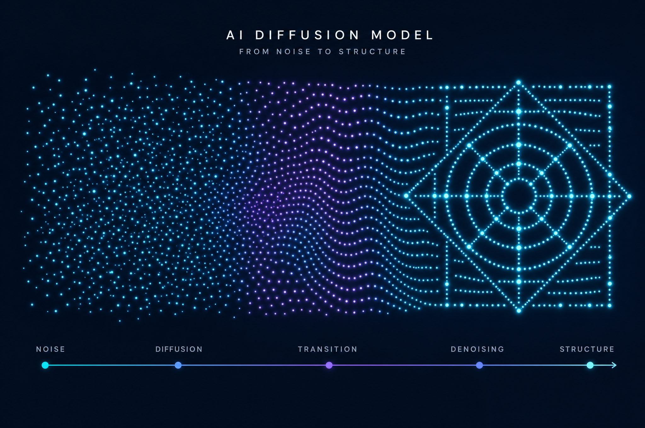
Stable Diffusion 1.5 was trained on over 2.3 billion image-text pairs. The compute cost has been estimated at roughly 150,000 GPU-hours on A100 chips — on the order of $600,000 in cloud compute at prevailing rates. And that is considered a relatively modest training run by modern standards. Why does teaching a model to remove noise from images require such staggering amounts of data and compute?
The answer is not that diffusion models are inefficient. It is that the task they are learning is genuinely, profoundly hard. The model must learn to reverse a stochastic process — to look at noise and infer what image might have produced it. This is not pattern matching. It is statistical inference over an astronomically large space of possible images. And doing that inference well requires enormous coverage of what images can look like.
The Training Objective: Simpler Than It Seems
On paper, the training objective for a diffusion model is almost disappointingly simple. The model is shown a noisy image and asked to predict the noise that was added. That's it. The loss function is typically mean squared error between the predicted noise and the actual noise that was added during the forward process.
This simplicity is deceptive. Predicting noise is equivalent to predicting the original clean image, because the noise is just the difference between the clean image and the noisy version. So when the model learns to predict noise, it is implicitly learning the structure of natural images — which configurations of pixels are likely and which are not. This is an enormous amount of knowledge compressed into a single prediction task.
Training works because the forward process is mathematically tractable: you can add noise at any step t directly from the clean image, without simulating all intermediate steps. The noise at step t is x_t = √α_t · x_0 + √(1-α_t) · ε, where ε is standard Gaussian noise. The model learns to predict ε from x_t. This "jump to any timestep" property is what makes training feasible at all.
Why Coverage Matters
The core reason diffusion models need so much data is coverage. The model is learning the probability distribution of natural images — an incredibly high-dimensional, complex distribution. To sample from this distribution accurately, the model needs to have "seen" examples covering the full diversity of images it might be asked to generate.
Consider what happens if the training data is biased. Early versions of Stable Diffusion were criticized for producing images that overwhelmingly depicted Western aesthetics, lighter-skinned faces, and European architecture. This was not a bug in the model architecture — it was a direct reflection of the training data, which was drawn from web crawls of image-text pairs and therefore overrepresented content from English-speaking, Western internet users. The model learned the distribution it was shown, including its biases.
This coverage problem is compounded by the curse of dimensionality. An image of 512×512 pixels with 3 color channels lives in a 786,432-dimensional space. Even in the compressed latent space of Stable Diffusion (64×64×4 = 16,384 dimensions), the space of possible configurations is astronomical. The manifold of natural images — the tiny subset of this space that looks like real photographs, paintings, or drawings — is complex and folded. Covering it adequately requires millions of examples.
The Role of Text Conditioning
The text-conditioned version of the problem is even harder. The model must learn not just what images look like, but the mapping from language to visual concepts. The phrase "a cat on a windowsill" must map to a region of image space containing cats, windowsills, and their spatial relationship. Each concept must be learned separately, and the combinations must be learned too.
This is why CLIP text encoders are pretrained on hundreds of millions of image-text pairs before being incorporated into the diffusion model. The text encoder provides the semantic structure; the diffusion model learns to map that structure to pixels. Without the pretrained encoder, the diffusion model would have to learn language and vision simultaneously — a far harder task.
The Compute Scaling Law
Empirically, diffusion models obey a scaling law: model quality improves predictably with more data and more compute, following roughly a power law. Each doubling of training data produces a measurable improvement in image quality, fidelity, and prompt adherence. But the returns are diminishing — you need exponentially more data for each incremental improvement.
This is why the largest models (like those from OpenAI, Google, and Midjourney) are trained on proprietary datasets that go far beyond what is publicly available. They use filtered, curated, and sometimes synthetic data to maximize the information per training example. The data pipeline — collection, filtering, deduplication, captioning — is as important as the model architecture, and often more secretive.
Why Not Fewer Images?
A natural question: why can't we train on fewer images and accept lower quality? The answer is that diffusion models are surprisingly sensitive to data quality and diversity. Train on too few images, and the model overfits — it memorizes specific training images rather than learning the general distribution. Generate from an overfit diffusion model and you'll get near-duplicates of training images, not novel compositions.
The goal of training is generalization: the ability to produce images that are plausible (they look real) but novel (they don't exist in the training set). Achieving this requires enough examples that the model can't simply memorize them all and is forced to learn the underlying distribution. This is the same principle that governs all machine learning, but the complexity of the image distribution makes the data requirements particularly large for diffusion models.
The Forward Process as Data Augmentation
One elegant feature of diffusion training is that the noise injection itself acts as a form of data augmentation. Each training image is shown to the model at many different noise levels — from barely noisy to almost pure static. This means each image contributes many training examples, each at a different point along the noise schedule. A single image might generate a thousand training samples across different noise levels and random noise instantiations.
This doesn't eliminate the need for large datasets — the underlying diversity of images still needs to be covered — but it does mean each image is used more efficiently than in a model that learns from each image once. The noise schedule effectively stretches each image across the entire range of denoising difficulties, from easy (low noise) to very hard (high noise).
The Cost of Generation
The training cost is a one-time expense. Once trained, the model can generate images indefinitely. But the generation cost — running the model for 20-50 denoising steps per image — is also nontrivial. Each step requires a full forward pass through the U-Net. This is why faster samplers (like DPM-Solver, which reduces steps to 10-20) and distillation techniques (training a smaller model to mimic a larger one) are active areas of research. They trade a small quality loss for a large speed gain.
For more on the generation side, see our article on how denoising works step by step, which traces exactly what happens during those 20-50 iterations.
What the Model Actually Learns
Despite the enormous data and compute, what the model learns is conceptually simple: a score function — the gradient of the log-probability of the data distribution. At any point in image space, the score function points toward higher-probability configurations. Following the score from random noise gradually moves you toward realistic images. This is the Fokker-Planck connection: the score function is the drift term in the reverse-time diffusion equation.
The model doesn't learn to store images. It learns a vector field — a set of directions that, when followed, lead from noise to structure. This is why diffusion models can generate images that don't exist in the training data: they're following the learned probability gradient, not retrieving stored examples. The gradient is smooth and generalizes to new combinations of concepts the model has seen separately but never together.
Data Is the Bottleneck
As model architectures mature and training techniques improve, data has become the primary bottleneck. The largest models are limited not by GPU availability or algorithmic innovation, but by the supply of high-quality, diverse, well-captioned images. This has led to increasing interest in synthetic data (generating training images with existing models), data curation (filtering for quality and diversity), and efficient training (getting more from less data through better noise schedules, loss weighting, and curriculum learning).
The economics are clear: the model that wins is often the one with the best data, not the best architecture. Stable Diffusion's open release democratized the architecture; what remains contested is the data pipeline. In this sense, diffusion models are a microcosm of the broader AI industry: the algorithms are increasingly open, but the data is the moat.
If you're new to diffusion models, start with our non-technical introduction. If you're interested in the physics that inspired the training mathematics, our article on the connection between physical and AI diffusion traces the lineage from Fick to modern machine learning.