How Stable Diffusion Actually Works: From Noise to Image

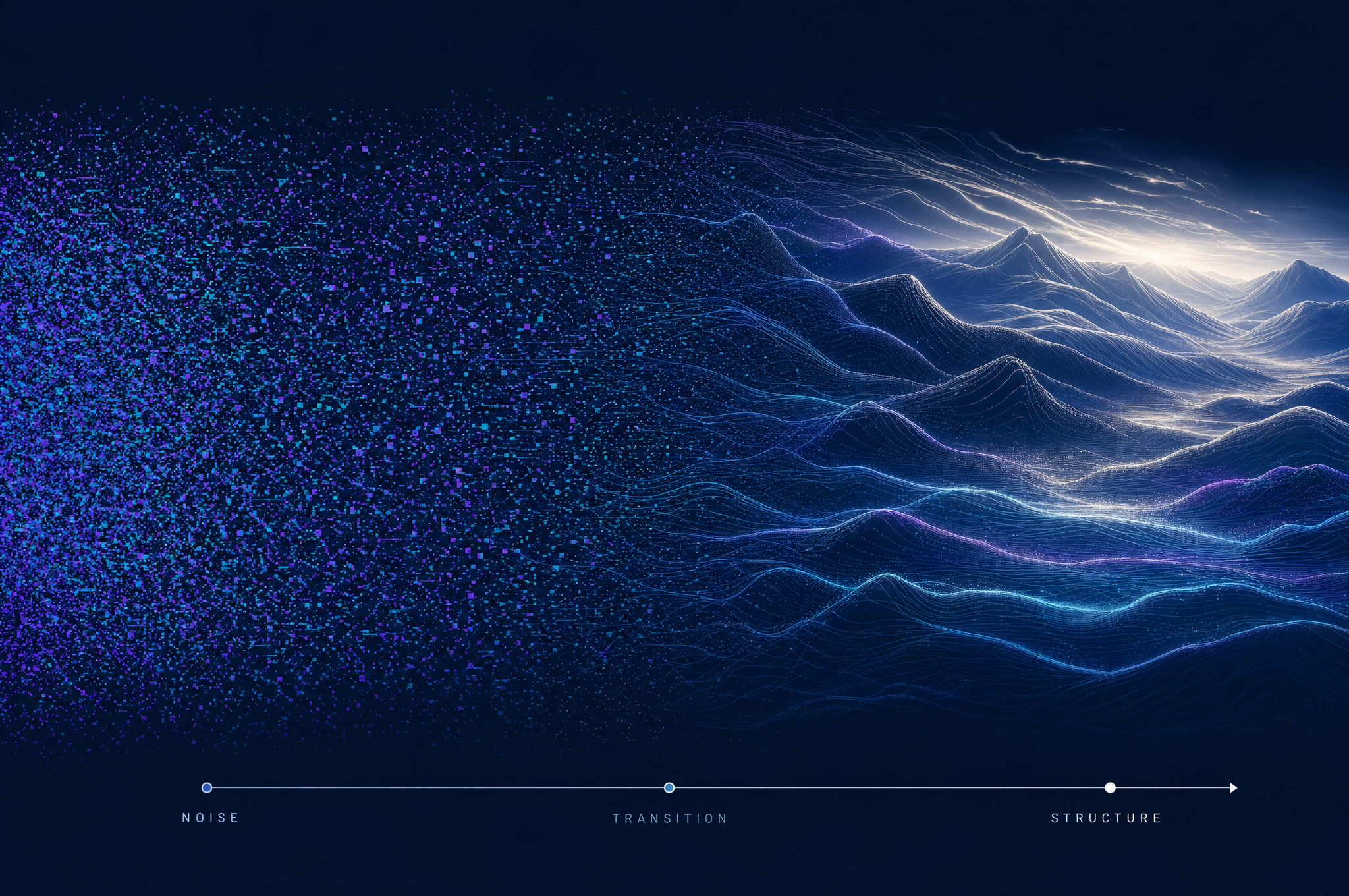
Stable Diffusion does not paint. It sculpts. It begins with a canvas of pure, unstructured noise — the kind of static you'd see on a dead television channel — and iteratively chisels away at that noise until a coherent image emerges. There is no brush. There is no pixel-by-pixel construction. There is only a repeated question: "What's the noise here, and what would this look like if I removed a little of it?"

That description is intuitive, but it hides enormous engineering complexity. Stable Diffusion is not a single model but an assembly of four distinct components, each trained separately and then wired together. Understanding how they cooperate is the key to understanding why Stable Diffusion is fast enough to run on a consumer laptop while producing images that rival systems running on data-center GPUs.

The Four Components

Before diving into the process, it helps to know the cast of characters. Stable Diffusion, released by the company Stability AI in 2022, combines four pieces:

• The Text Encoder (CLIP): Translates your text prompt into a numerical representation the model can understand.
• The VAE (Variational Autoencoder): Compresses images into a small latent representation and expands them back. This is the speed trick.
• The U-Net: The heart of the system. A neural network that predicts and removes noise, guided by the text.
• The Scheduler: The conductor that orchestrates the denoising loop, deciding how many steps to take and how aggressive each step should be.

Each of these deserves its own explanation, but the real magic happens when they work together. Let's trace the full pipeline from the moment you type a prompt to the moment an image appears on your screen.

Step 1: Encoding the Prompt

When you type "a cat sitting on a windowsill at sunset," the text is meaningless to the U-Net — it only understands numbers. The text encoder, based on OpenAI's CLIP model, converts your sentence into a sequence of vectors. Each vector captures the semantic meaning of a word or subword, along with its relationship to the other words in the sentence.

These vectors are not a simple lookup. CLIP was trained on hundreds of millions of image-text pairs, so its representations encode visual as well as linguistic meaning. The vector for "sunset" doesn't just mean "the sun goes down" — it carries information about warm colors, low angles, long shadows, and the visual texture of a sky at dusk. This rich, vision-aware embedding is what allows the model to generate images that match your intent rather than just illustrating the words literally.

Step 2: Starting in Latent Space

This is where Stable Diffusion diverges from earlier diffusion models like DALL-E 2 or Imagen. Those models performed diffusion directly in pixel space — they added and removed noise from a full-resolution image, pixel by pixel. A 512×512 image has 262,144 pixels, each with three color channels. Running a neural network over that space, hundreds of times, is enormously expensive.

Stable Diffusion's breakthrough was to move the entire diffusion process into a compressed latent space. The VAE encoder takes a 512×512 image and compresses it to a 64×64 representation with four channels — a 48x reduction in data. All the noise-adding and noise-removing happens in this tiny latent space, and only at the very end does the VAE decoder expand the result back to full resolution.

This is why Stable Diffusion can run on a consumer graphics card with 8 GB of VRAM while earlier models required multi-GPU setups. The U-Net is doing the same mathematical work, but on a representation that is 48 times smaller.

Step 3: The Denoising Loop

Now the main event begins. The system generates a tensor of pure Gaussian noise — random values drawn from a bell curve — in the latent space. This noise is the raw material from which the image will be carved. Think of it as a block of marble: the sculpture is already inside it, in a statistical sense, and the model just needs to remove what doesn't belong.

The scheduler determines how many steps the process will take. A typical generation uses 20 to 50 steps, though faster schedulers like DPM-Solver can produce good results in as few as 10. At each step, the following happens:

1. The U-Net takes the current noisy latent and the text embedding as inputs.
2. It predicts the noise component — an estimate of which parts of the latent are signal and which are noise.
3. The scheduler subtracts a fraction of the predicted noise from the latent.
4. The result becomes the input for the next step.

This is the same fundamental operation we described in our non-technical explanation of diffusion models: predict the noise, remove a little of it, repeat. But the details matter. The U-Net doesn't just predict raw noise — it predicts the noise conditional on the text. At every step, the text embedding steers the denoising toward images that match the prompt. The text is not a filter applied at the end; it is a force that shapes every single step of the process.

Step 4: The U-Net's Architecture

The U-Net deserves a closer look, because it is where most of the computational cost lives. Its name comes from its shape: the network first downsamples the latent (compressing spatial information into richer feature channels), then upsamples it back (restoring spatial resolution). The "U" shape allows it to capture both fine-grained local detail and broad spatial context.

At each resolution level, the U-Net applies attention layers that let different regions of the latent "talk" to each other. Cross-attention layers also inject the text embedding at every level, ensuring the prompt influences the image at all scales — from the overall composition down to the texture of individual features. This multi-scale attention is why the model can get global composition right (the cat is on the windowsill) while also rendering local detail (the cat has fur, the window has a frame).

Step 5: Decoding to Pixels

After the final denoising step, the latent contains a clean, structured representation of the image — but it is still in compressed form. The VAE decoder takes this latent and expands it back to full 512×512 resolution. This is a single forward pass, fast and deterministic. The image you see is the decoder's interpretation of the latent.

One consequence of this architecture is that the VAE imposes a quality ceiling. The diffusion process can produce a perfect latent, but if the decoder can't faithfully reconstruct the details, the final image will be blurry or artifact-prone. This is why later versions of Stable Diffusion shipped improved VAEs — the diffusion model hadn't changed, but the decoder was better at translating latents into sharp pixels.

The Role of the Scheduler

The scheduler is an underappreciated component. It determines how much noise to remove at each step, and different schedulers make different trade-offs. Some, like DDIM (Denoising Diffusion Implicit Models), remove noise in a way that allows fewer steps without quality loss. Others, like Euler ancestral, introduce stochasticity at each step, producing more varied (but less reproducible) results.

The scheduler also controls a parameter called guidance scale, or CFG (Classifier-Free Guidance). This scales how strongly the text embedding pulls the denoising toward the prompt. A guidance scale of 1 means the model follows the prompt loosely; a scale of 7-12 (the typical default) means it follows the prompt aggressively. Too high, and the image becomes oversaturated and distorted — the model overcommits to the prompt at the expense of natural appearance. Too low, and the image ignores the prompt entirely.

Why It's Called "Stable"

The name "Stable Diffusion" refers to Stability AI, the company that funded the compute for training. But there's a double meaning: diffusion models are inherently more stable to train than the GANs they replaced. GAN training was a two-player game between a generator and a discriminator, and if the balance tipped, the whole system could collapse. Denoising diffusion models have a simple, well-behaved training objective: predict the noise. No adversarial game, no delicate balance, no mode collapse. The training is stable enough that the model converges reliably even at massive scale.

From Noise to Meaning

What makes Stable Diffusion remarkable is not any single component but the way they compose. The text encoder provides intent. The VAE provides efficiency. The U-Net provides the core skill of denoising. The scheduler provides control over speed and style. Together, they turn a string of text and a block of random noise into an image that didn't exist a moment before.

If you want to understand the training process that gives the U-Net its denoising ability, read our deep dive on why diffusion models need so much data. And if you're curious about the mathematical roots of the entire approach — why the same equations that describe ink spreading through water also describe noise being added to an image — our article on the Fokker-Planck equation is the place to start.