Denoising Diffusion: How AI Learns to Remove Noise Step by Step

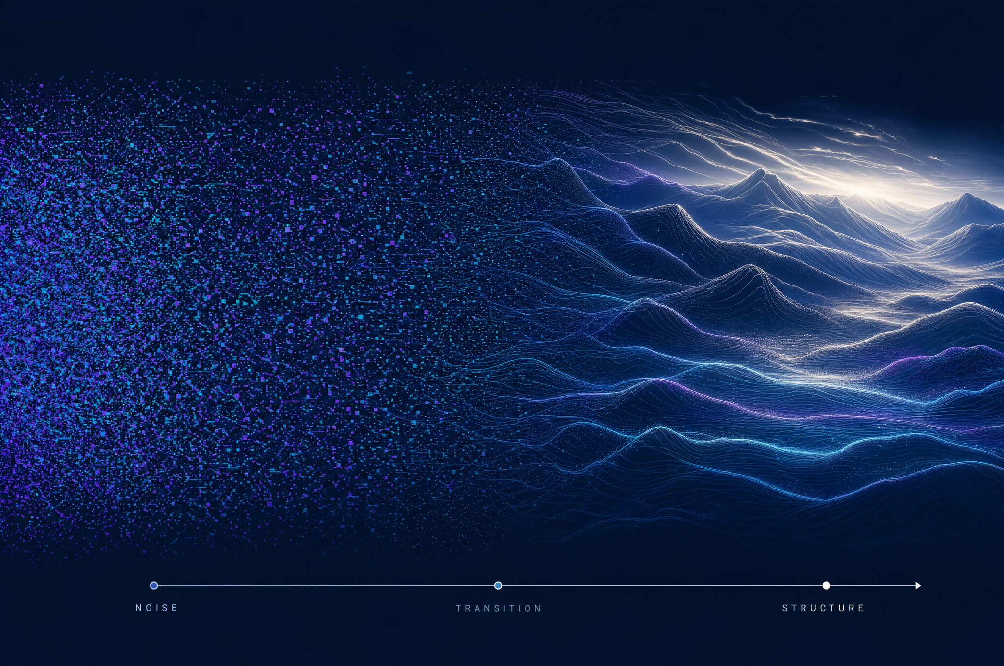
There is a peculiar elegance in the training objective of a denoising diffusion probabilistic model. The network never learns to generate an image. It never learns composition, color theory, or perspective. It learns exactly one thing: given a noisy image, predict the noise. Remove that predicted noise, and you have a slightly cleaner image. Repeat the process dozens of times, and you have transformed pure static into a photograph. The complexity of image generation emerges from the repetition of a single, simple act.

This is the core insight of DDPMs — denoising diffusion probabilistic models — introduced by Jonathan Ho, Ajay Jain, and Pieter Abbeel in 2020. Their paper, building on earlier work by Jascha Sohl-Dickstein, showed that a well-trained denoising network, iterated over enough steps, could produce images of stunning quality. The approach was so effective that it became the foundation for virtually every modern image generation system, from Stable Diffusion to DALL-E 3 to Midjourney.

The Training Procedure

Training a DDPM is conceptually straightforward, even if the engineering is demanding. The process works as follows:

1. Take a clean image from the training set.
2. Pick a random timestep t between 1 and T (typically T = 1000).
3. Add noise to the image corresponding to timestep t. Thanks to the mathematical properties of Gaussian noise, you can jump directly to any timestep without simulating the intermediate steps.
4. Ask the neural network to predict the noise that was added.
5. Compute the loss: the mean squared error between the predicted noise and the actual noise.
6. Backpropagate and update the network weights.

That's it. The network sees the same images at many different noise levels — from barely noisy (small t) to almost pure static (large t). Over millions of training examples and billions of gradient updates, the network learns to predict noise at every level of corruption.

The Noise Schedule

A critical design choice is the noise schedule — how much noise is added at each timestep. Early schedules (like the one in the original DDPM paper) used a linear schedule: the variance increased linearly from step 1 to step T. Later work found that cosine schedules, which add noise more slowly at the beginning and end, produce better results because they give the model more training signal at the noise levels that matter most for image quality.

The noise schedule matters because it determines what the network sees during training. If too many training examples are at very high noise levels (where the image is essentially destroyed), the network spends its capacity learning to predict noise from pure static — a trivial task, since the noise is the entire signal. If too many examples are at very low noise levels, the network never learns to handle the difficult high-noise regime. A good schedule balances these, concentrating training signal where the model needs it most.

The U-Net: The Denoising Engine

The neural network that performs the denoising is almost always a U-Net — an architecture originally developed for medical image segmentation. The U-Net takes the noisy image and the timestep t as inputs and outputs a prediction of the noise. The timestep is critical: the network must know how noisy the image is, because the optimal denoising strategy differs at each noise level.

The U-Net's encoder-decoder structure, with skip connections, allows it to capture both fine spatial detail (through the decoder's high-resolution path) and broad contextual understanding (through the encoder's low-resolution path). When text conditioning is added — as in Stable Diffusion — cross-attention layers inject the text embedding at multiple points, allowing the prompt to influence denoising at every scale.

The Sampling Loop: Generating Images

Once trained, the model generates images by running the denoising process in reverse. Starting from pure Gaussian noise at timestep T, the model repeatedly:

1. Predicts the noise at the current timestep.
2. Subtracts a fraction of the predicted noise (the fraction is determined by the scheduler).
3. Adds a small amount of fresh random noise (this stochasticity is important — see below).
4. Moves to the next-lower timestep and repeats.

After T steps (or fewer, with modern fast samplers), the result is a clean image sampled from the learned distribution. The entire generation process is a Markov chain running in reverse — each step depends only on the current state, not on the history of how it got there.

Why Stochasticity Matters in Sampling

One non-obvious aspect of DDPM sampling is that each step adds a small amount of fresh noise, even as it removes the predicted noise. This seems counterintuitive — why add noise when the goal is to remove it? The answer lies in the mathematics of the reverse diffusion process.

The forward process adds Gaussian noise at each step. The reverse process must undo this, and because Gaussian noise is involved, the reverse step has a deterministic component (the predicted mean) and a stochastic component (the residual variance). Skipping the stochastic component produces lower-quality images because it ignores the full distribution of possible reverse transitions. The added noise ensures the sampling process explores the full probability distribution rather than collapsing to a single mode.

This is where DDPMs connect to the Langevin equation from physics. The sampling loop is, mathematically, a discretized Langevin dynamics simulation — the same stochastic process that describes the motion of a particle in Brownian motion. The model provides the drift (the score function, pointing toward higher probability), and the added noise provides the diffusion. Together, they trace a path through image space that converges to the data distribution.

The Score Function Connection

Under the hood, predicting noise is equivalent to estimating the score function — the gradient of the log-probability of the data distribution. At any point in image space, the score function points in the direction of increasing probability. Following the score from random noise gradually moves you toward regions of high probability — toward realistic images.

This equivalence, shown by Yang Song and Stefano Ermon in their work on score-based generative models, unified two apparently different approaches: DDPMs (which frame the problem as reversing a noise-adding process) and score-based models (which frame it as following the gradient of a probability density). The two are mathematically identical. The noise prediction network is learning the score, and the sampling loop is Langevin dynamics following that score.

This connection to the score function is what links diffusion models to the Fokker-Planck equation. The score is the drift term in the reverse-time Fokker-Planck equation. The entire generative process can be written as a stochastic differential equation — the same type of equation that describes physical diffusion. We explore this deep connection in our article on the relationship between physical and AI diffusion.

From DDPM to Modern Models

The original DDPM required 1000 steps to generate an image — far too slow for practical use. The field has since developed numerous acceleration techniques:

• DDIM (Denoising Diffusion Implicit Models): A deterministic sampling method that skips steps without quality loss, reducing generation to 20-50 steps.
• DPM-Solver: A specialized ODE solver for diffusion equations that achieves good results in 10-20 steps.
• Latent diffusion: Moving the process into compressed latent space (the key innovation of Stable Diffusion), which makes each step faster.
• Distillation: Training a student model to mimic the multi-step teacher in fewer steps, sometimes as few as 1-4.

Despite these accelerations, the fundamental principle remains the same: the model predicts noise, the scheduler removes it, and repetition transforms static into structure. Every modern image generator — from open-source Stable Diffusion to proprietary systems — is a variation on this theme.

The Power of a Simple Skill

What makes denoising diffusion so powerful is that it decomposes an impossibly hard problem — generate a realistic image from scratch — into a very large number of very easy problems — remove a little bit of noise. Each individual denoising step is a simple regression task. The network doesn't need to understand global composition in a single pass. It just needs to make a local correction. The global structure emerges from the accumulation of thousands of such corrections, each guided by the text prompt and the learned probability distribution.

This is why diffusion models are more stable than the GANs they replaced. GANs had to learn to generate an image in a single forward pass — a high-dimensional, adversarial problem that was prone to failure modes like mode collapse. Diffusion models break the problem into manageable pieces, and each piece is a simple, well-behaved supervised learning task. The complexity is in the iteration, not in any single step.

If you want to understand the broader context, start with our non-technical introduction to diffusion models or our deep dive on why training requires so much data. The story of how a single, simple denoising skill became the most powerful approach to image generation is one of the most elegant chapters in the history of AI.