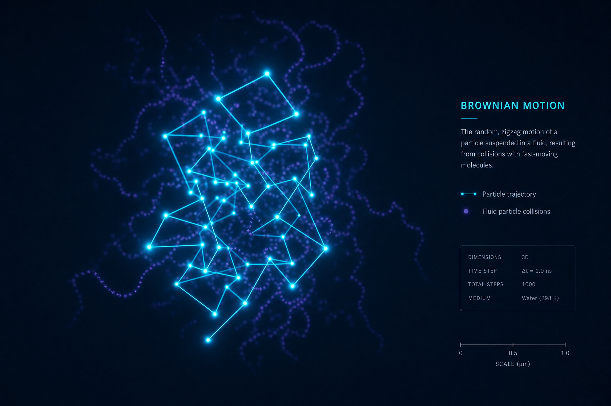
If you track a single particle undergoing Brownian motion, its path is a jagged, unpredictable mess. No equation can tell you where it will be at any given moment. But if you track a million particles, the picture changes entirely. The cloud spreads smoothly, predictably, and its shape follows an exact mathematical law. That law is the Fokker-Planck equation.
The Fokker-Planck equation is the bridge between the chaotic microscopic world of individual random walks and the orderly macroscopic world of diffusion. It is the equation that tells you, not where any single particle will go, but how the probability of finding a particle at any given point evolves over time. And remarkably, the same equation that describes ink spreading through water also describes how noise accumulates in an AI diffusion model during training.
From Particles to Probability
To understand the Fokker-Planck equation, we need to shift our perspective. Instead of asking "where is this particle?" we ask "what is the probability of finding a particle at position x at time t?" This shifts us from tracking individual trajectories to tracking a probability density — a function p(x, t) that tells us how probability is distributed across space at any moment.
For a purely deterministic process — say, a ball rolling downhill — the probability density is a spike that moves along the trajectory. But for a stochastic process, the probability density spreads out. A particle starting at the origin doesn't stay at the origin; it wanders. Over time, the probability of finding it near the origin decreases, and the probability of finding it farther away increases. The Fokker-Planck equation tells us exactly how that spreading happens.
Two Forces: Drift and Diffusion
The equation gets its power from separating two distinct influences on the particle's motion: drift and diffusion.
Drift is a systematic force that pushes particles in a preferred direction. Gravity pulling a sedimenting particle downward is drift. An electric field pulling an ion is drift. In the Fokker-Planck equation, drift appears as a term involving the first derivative of the probability density — it describes how the peak of the distribution moves over time.
Diffusion is the spreading caused by random thermal motion. Even with no drift at all, a cloud of particles will spread because each particle is randomly jostled. Diffusion appears as a term involving the second derivative — it describes how the distribution widens, regardless of where its center is.
The Fokker-Planck equation says: the rate of change of probability equals the negative divergence of the drift flux, plus the diffusion of the probability itself. In one dimension: ∂p/∂t = -∂/∂x [A(x)p] + ½ ∂²/∂x² [B(x)p], where A(x) is the drift coefficient and B(x) is the diffusion coefficient. The first term moves probability; the second term spreads it.
That's the entire equation. It looks compact, but it contains worlds. The drift term A(x) can be any function of position — constant gravity, a varying electric field, the curvature of a potential energy landscape. The diffusion term B(x) can also vary, reflecting changes in temperature or viscosity. Together, they describe the complete evolution of the probability distribution.
The Connection to Fick's Laws
If you strip away the drift term entirely — set A(x) to zero — the Fokker-Planck equation reduces to something familiar. It becomes ∂p/∂t = D ∂²p/∂x², which is exactly the diffusion equation that Fick derived in 1855. In this special case, the probability density is just the concentration of particles, and the equation says that concentration changes in proportion to how sharply it varies in space — the steeper the gradient, the faster the spreading.
This is not a coincidence. Fick's laws are a special case of the Fokker-Planck equation — the case with no drift and constant diffusion. The Fokker-Planck equation is the generalization: it adds drift, allows the diffusion coefficient to vary, and applies to any probability distribution, not just particle concentration. Fick described what happens when particles spread with no external force. Fokker and Planck described what happens when forces and randomness coexist.
The Langevin Equation: The Other Side
The Fokker-Planck equation has a companion: the Langevin equation. Where the Fokker-Planck equation describes the probability distribution, the Langevin equation describes individual particle trajectories. It writes the motion of a particle as a sum of a deterministic drift term and a random noise term:
dx = A(x) dt + √B(x) dW
Here, dW is a Wiener process — the mathematical formalization of Brownian motion. Each tiny step the particle takes is partly determined by the drift A(x) and partly random, with the magnitude of the randomness set by B(x). The Langevin equation and the Fokker-Planck equation are two descriptions of the same process: one tracks individuals, the other tracks populations. They are mathematically equivalent — you can derive one from the other.
Why This Equation Appears Everywhere
The Fokker-Planck equation shows up in an astonishing range of fields because any system that combines deterministic forces with randomness is governed by it. In physics, it describes the motion of charged particles in a plasma, the relaxation of spins in nuclear magnetic resonance, and the folding of proteins. In chemistry, it describes reaction rates in solution, where molecules must diffuse together before they can react. In finance, it appears (in disguise) as the Black-Scholes equation, where stock prices play the role of particles and volatility plays the role of diffusion.
In biology, the Fokker-Planck equation describes how signaling molecules spread across a tissue, how populations evolve under genetic drift, and how ions distribute across membranes. The transport of molecules across cell membranes, which keeps cells alive, is governed by precisely this interplay of drift (the electrical potential across the membrane) and diffusion (the thermal motion of ions).
The Bridge to AI
Here is where the story takes a surprising turn. When AI researchers build denoising diffusion models, they are — knowingly or not — working with the Fokker-Planck equation. The forward process in a diffusion model adds Gaussian noise to an image step by step. This is a stochastic process governed by a Langevin equation, and the corresponding probability distribution evolves according to a Fokker-Planck equation.
The forward process gradually transforms any initial image distribution into pure Gaussian noise. The reverse process — the generative process — must run the Fokker-Planck equation backward in time. This is where a deep result from stochastic calculus enters: under certain conditions, the reverse-time process is also governed by a Fokker-Planck equation, but with a modified drift term that depends on the gradient of the log-probability, known as the score function.
The score function ∇ log p(x) tells you which direction increases the probability density. In a diffusion model, the neural network is trained to approximate this score — to point from any noisy image toward higher-probability (less noisy) configurations. Reversing the Fokker-Planck equation with this score as drift is what generates images from noise.
This is why diffusion models are called diffusion models. It is not a metaphor. The forward process is a Fokker-Planck diffusion. The reverse process is a Fokker-Planck diffusion with a learned drift. The mathematics is the same mathematics that Adolf Fick used to describe ink in water and that Albert Einstein used to prove atoms exist. We explore this connection in full in our article on the connection between physical and AI diffusion.
Solving the Equation
The Fokker-Planck equation is a partial differential equation, and like most PDEs, it rarely has a closed-form solution. For simple cases — constant drift, constant diffusion — the solution is a Gaussian that moves and spreads over time. For more realistic scenarios, physicists and engineers rely on numerical methods: finite difference schemes, spectral methods, or, increasingly, the Langevin equation itself, simulated by drawing random numbers.
This last approach — simulating many Langevin trajectories and averaging them — is called a Monte Carlo method, and it is the practical workhorse of stochastic modeling. It is also, in a beautiful recursion, exactly how diffusion models generate images: they simulate the reverse-time Langevin equation, drawing random numbers at each step, and the resulting trajectory produces a sample from the image distribution.
An Equation That Connects Disciplines
The Fokker-Planck equation is rare in science: a single piece of mathematics that is simultaneously fundamental to physics, chemistry, biology, finance, and artificial intelligence. It describes how probability spreads under the joint influence of determinism and chance. Whether the "particles" are ink molecules, stock prices, or pixels in a neural network, the equation is the same. Understanding it is understanding diffusion at its most general — and most powerful.
To see the equation in its simplest form, start with Fick's laws. To see its most dramatic application, read about Brownian motion and how it proved the existence of atoms. And to see where it goes next, read about how the same mathematics now powers the AI that generates images from text.